Incremental efficient frontier

Step 1: Efficient frontier

First let’s write a simple code for an efficient frontier computation

efficient_frontier = function(MRet                         #matrix of returns (MRet)
                              , rangeMu)                   #range (sequence) of target expected returns (rangeMu)
{
                                              
  uM <- dim(MRet)[1]                                       #get the row (uM) and column (pM) dimensions of the matrix of returns
  pM <- dim(MRet)[2]
  
  expRet <- colMeans(MRet)                                 #compute the portfolio's individual stocks expected returns

  Omega = var(MRet)                                        #compute the sample var-covar matrix

  unityVec <- rep(1, pM)                                   #define a constraints vector (weights of the portfolio must sum to one)
  
  A <- rbind(expRet, unityVec)                             #define a matrix of constraints (weights sum to one and variance will match a                                                                   #target level of expected returns)        

  n <- length(rangeMu)                                     #get the length of the target range (sequence)
  
  myVar <- rep(NA, n)                                      #define an empty variance vector
  
  myWeights <- matrix(data = NA, nrow = n, ncol = pM)      #define an empty matrix of weights for each stock at each level of target
                                                           #expected returns
  
 
  for(i in 1:n)                                            #loop over the target expected returns range and compute variances and weights 
  {                                                        
    b <- matrix(data = c(rangeMu[i], 1), nrow = 2)
    myVar[i] <- t(b) %*% solve(A %*% solve(Omega) %*% t(A)) %*% b
    myWeights[i,] <- solve(Omega) %*% t(A) %*% solve(A %*% solve(Omega) %*% t(A)) %*% b
  }

  mySd <- myVar^0.5                                        #compute the standard deviation vector
  
  return(mySd)                                             #return the standard deviation vector
}

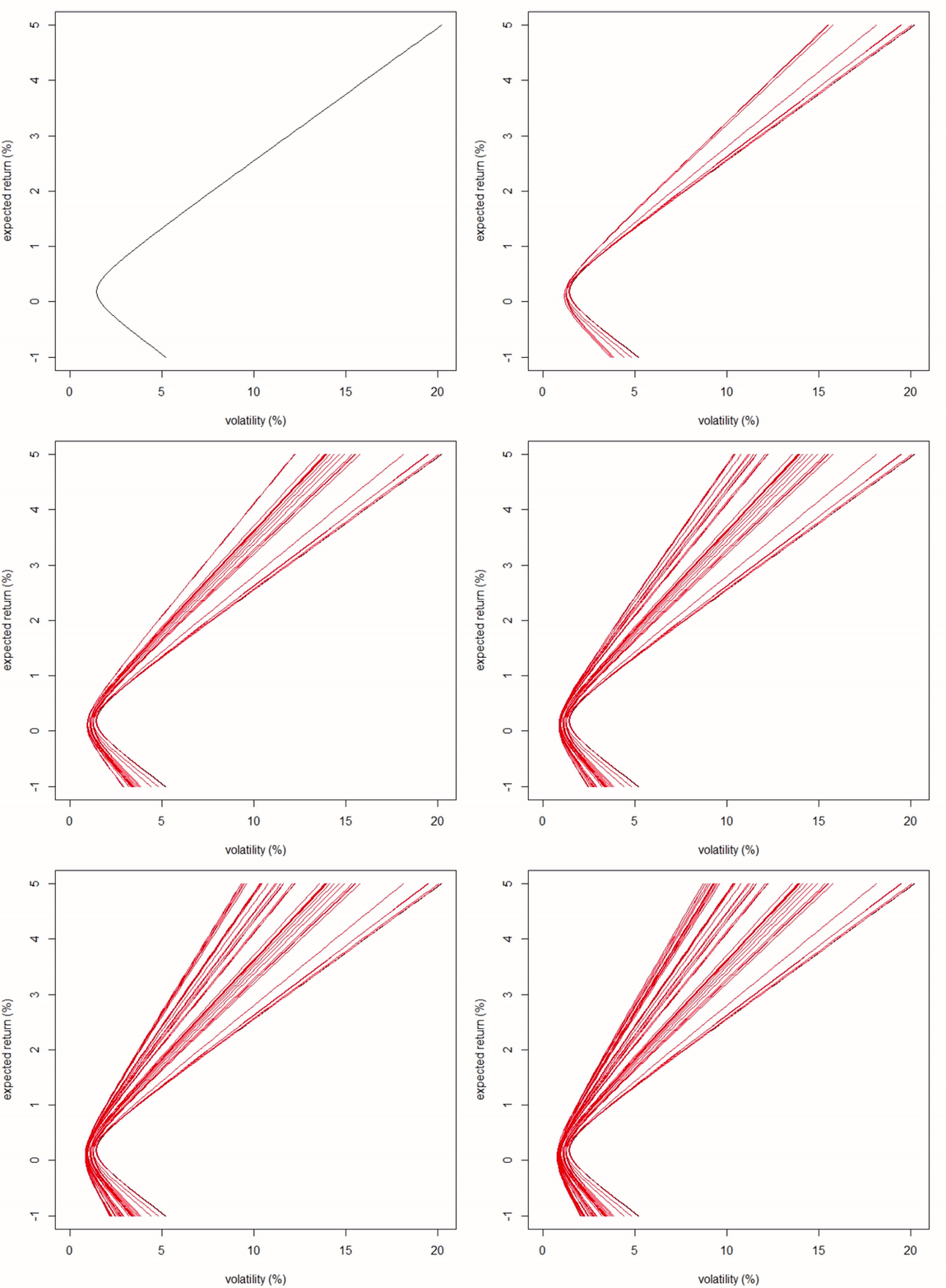
Step 2: Incremental efficient frontier

efficient_frontier_increment = function(MRet)                      #define a function that takes as argument a matrix of returns (MRet)
{
  pM <- dim(MRet)[2]                                               #get the column (pM) dimension of the matrix of returns
  
  rangeMu <- seq(-0.01, 0.05, 0.001)                               #hard code the vector of expected returns (can be passed as argument)
  
  mySd <- efficient_frontier(MRet[, 1:9], rangeMu)                 #compute the sd vector of the portfolio composed of the first nine stocks  
  
  
  dev.new()                                                        #get a new plot
 
  plot(mySd * 100                                                  #plot the efficient frontier of the portfolio composed of the first 9 stocks
       , rangeMu * 100
       , xlab = "volatility (%)"
       , ylab = "expected return (%)"
       , t = 'l'
       , xlim = c(0, max(mySd * 100))
       , ylim = c(-1, 5))   
  
  Sys.sleep(2)                                                     #enjoy the chart for two seconds
  
  for(j in 10:pM)                                                  #loop over all stocks and increment the portfolio with the next stock
  {
    mySd <- efficient_frontier(MRet[, 1:j], rangeMu)               #recompute the efficient frontier
    
    lines(mySd * 100, rangeMu * 100, col = 'red')                  #add a line of the more efficient frontier on the chart
    
    Sys.sleep(0.1)                                                 #define how long you want to wait before the next one
  }
}

Result in animation

Fig 1. Animation of an efficient frontier with stock increment

To run the code with real historical figures, I propose a *.csv file of NYSE returns Download nyse_stocks_historical_returns.csv