Inefficiency of markets with negative prices?
In this post, I briefly describe the event of negative prices market which occured on the NYMEX WTI crude oil May contract
Event description
On April 15, 2020, the CME clearing released an advisory notice mentioning the possibility of negative prices in some NYMEX energy contracts. They indicate that their environment and message format are ready to handle such situation, see the CME advisory notice. On April 20, 2020, at the end of the trading day and one day before the contract expires, the May futures contract written on WTI crude oil and traded on NYMEX reached the negative territory for the first time and even dropped to -40.32 USD / barrel.
Dataset description
Once the event began it took me about two hours to write a recording algorithm which connected to the NYMEX and started to record all the trading messages (I missed the beginning of the journey in this southern territory). The 12 hours of recording still represents over five million observations with the full book records of levels and quantities, as well as all buyer and seller initiated orders. The time stamps have a hundred nanoseconds granularity (one ten-millionth a second and corresponds to the time elapsed since midnight of January 1, 2001). For complete accuracy, you should add about 54 milliseconds, the average half-ping that I get from my University server to Aurora, Illinois. where the exchange server is located. The first column of the dataset is the time-stamp, the two next columns are the best ask and bid levels, the two next are the best ask and bid quantities and the two last are the cumulative buyer and seller initiated orders. The raw dataset also includes the matching order book data for the June and July contracts. I clean them out and only keep each observations that represents a change in the top of the book of the May contract.
Descriptive price plot
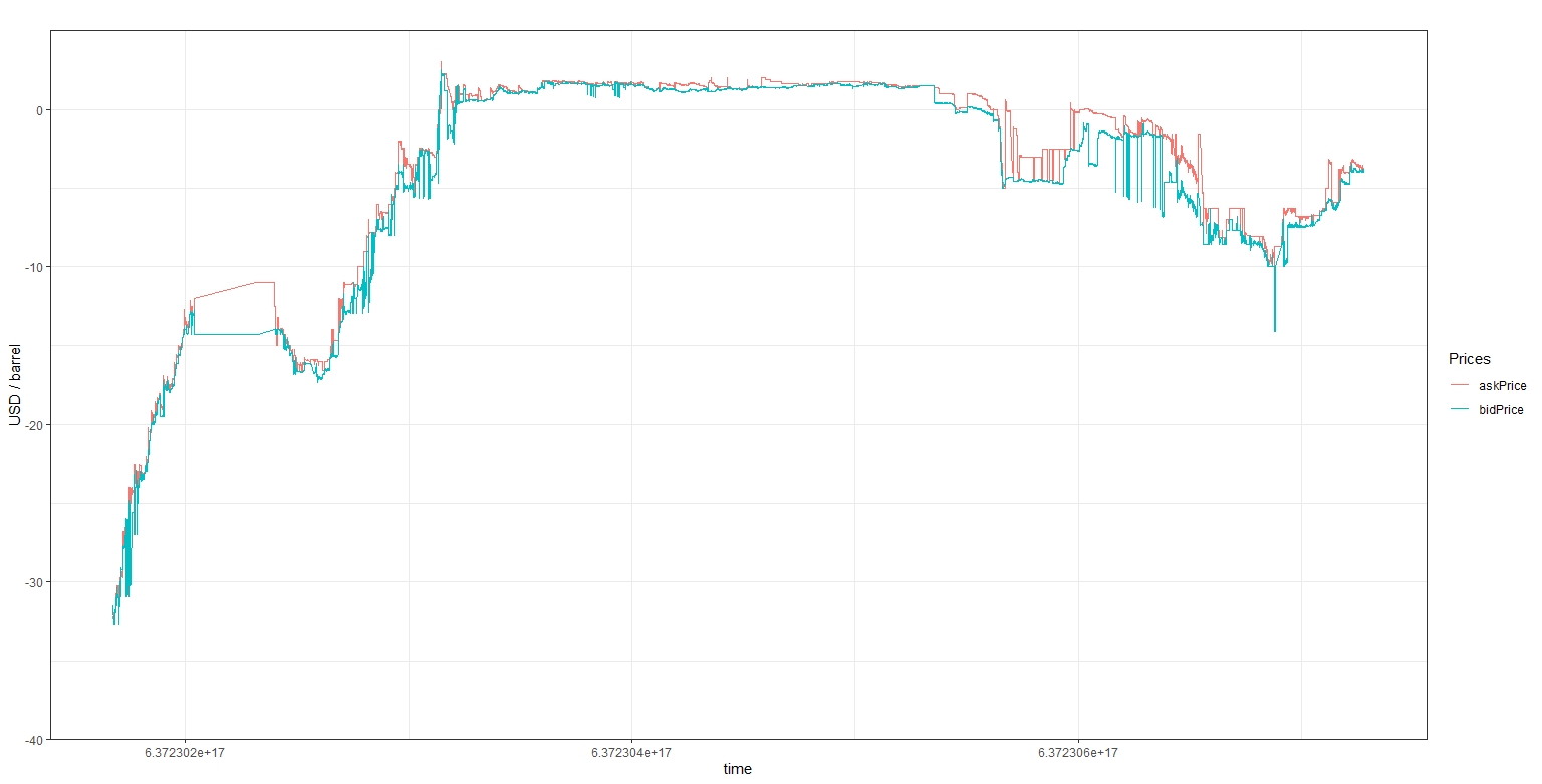
Fig 1. Ask and bid prices plot between April 20 and 21, 2020.
Code
plot_crude <- function()
{
  library(ggplot2)
  library(reshape2)
  X <- read.csv("C:/yourPathToFile.csv", stringsAsFactors = FALSE)

  #get the dimensions
  uX <- dim(X)[1]
  pX <- dim(X)[2]

  #get the variables
  timeStamp <- X[, 1]
  askPrice <- X[, 2]
  bidPrice <- X[, 3]

  askSize <- X[, 4]
  bidSize <- X[, 5]

  volumeBought <- X[, 6]
  volumeSold <- X[, 7]

  #create a data frame for the prices
  priceDf <- data.frame(cbind(timeStamp, askPrice, bidPrice))
  colnames(priceDf) <- c("timeStamp", "askPrice", "bidPrice")

  priceDf <- melt(priceDf, id.var = "timeStamp")                                   #reshape to long format
  colnames(priceDf)[2] = "Prices"
  colnames(priceDf)[1] = "timeStamp"

  dev.new()
  g1 <- ggplot(priceDf, aes(x = timeStamp, y = value, group = Prices, colour = Prices))
  g1 <- g1  + geom_line()

  g1 <- g1 + ggtitle("") + xlab("time") + ylab("USD / barrel")

  g1 <- g1 + coord_cartesian(ylim = c(-40, 5))
  g1 <- g1 + scale_y_continuous(expand = c(0,0))
  g1 <- g1 + theme_bw()
  return(g1)
}
A focus on the beginning of the event
Zooming on the plot, it appears that at the beginning of the recorded dataset some bid and ask quoted prices experienced an inversion. It is possible that the matching algorithm (or the data sent over by the exchange) did not really handle the negative prices. In the plot below I represent the absolute bid-ask spread (in USD / barrel). Note that there is a long period when I received no quotes (again, it does not mean the exchange stopped).
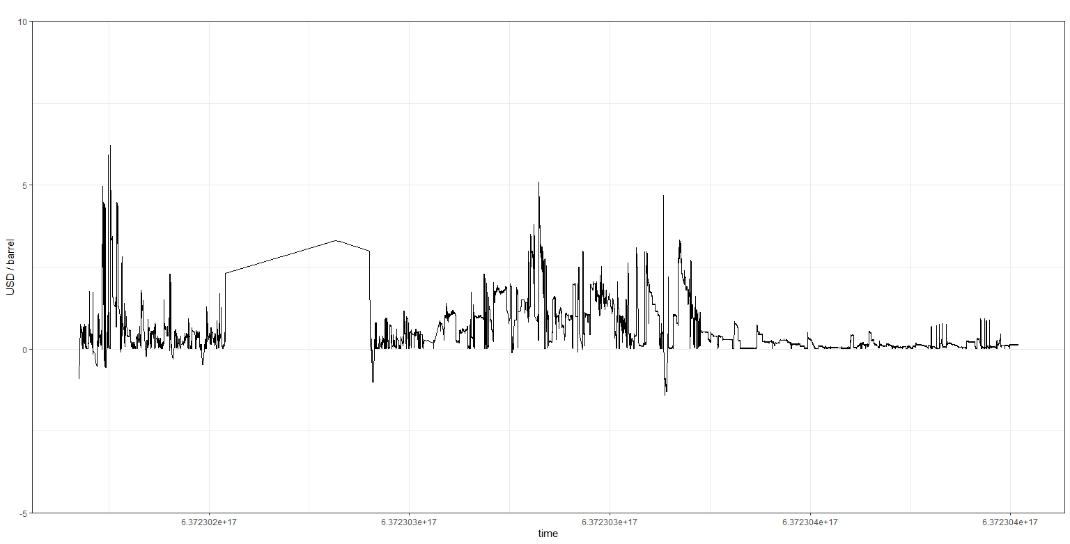
Fig 2. Absolute bid-ask spread during the end of April 20 2020 session.
Code
  #Just change the code above to:
  spread <- askPrice - bidPrice
  #create a data frame for the prices and spread  and restrict the dataset to the beginning of the event
  priceDf <- data.frame(cbind(timeStamp, askPrice, bidPrice, spread))[1:(uX / 5), ]
  colnames(priceDf) <- c("timeStamp", "askPrice", "bidPrice", "spread")

  dev.new()
  g1 <- ggplot(priceDf, aes(x = timeStamp, y = spread))
How long did these events last, and how much risk-free profit there was left?
Running the code below provides both en estimate of the average opportunity time, an important aspect if, like me, you attempt to trade with a > 100 ms ping and how much cumulative profit and loss these inverted bid-ask spread could generate. Interestingly, when I compute the average inverted bid-ask spread I obtain an average time of 24.5 seconds (more than enough to arbitrage the market). However, I find that no trades occured during these conditions. My guess is that the matching engine turned off which explains why the bids and asks crossed!
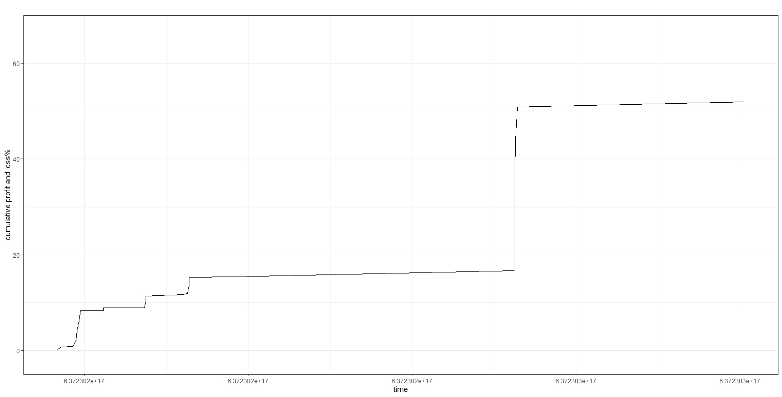
Fig 3. Profit and loss potential of the May WTI crude oil April 20 2020 session.
Code
pnl_crude_spread <- function()
{
  library(ggplot2)
  library(reshape2)
  X <- read.csv("C:/yourPathToFile.csv", stringsAsFactors = FALSE)

  #get the dimensions
  uX <- dim(X)[1]
  pX <- dim(X)[2]

  #limit the test to the beginning of the event.
  X <- X[1:(uX / 5), ]
  uX <- dim(X)[1]

  #get the variables
  timeStamp <- X[, 1]
  askPrice <- X[, 2]
  bidPrice <- X[, 3]

  askSize <- X[, 4]
  bidSize <- X[, 5]
  spread <- askPrice - bidPrice

  #get the volume bought and sold at each tick (differentiate as it is recorded cumulatively)
  volumeBought <- c(0, diff(X[, 6]))
  volumeSold <- c(0, diff(X[, 7]))
  volumeTotal <- volumeBought + volumeSold

  pnl <- rep(0, uX)
  timeInvertSpread <- NA
  timeStart <- 0


  #maximum possible trading size given the best bid best ask size
  maxSize <- 0
  #loop over the data
  for(i in 2:uX)
  {
    #condition on whether the bid ask spread started to be negative or equal to zero (theoretically impossible)
    if(spread[i] <= 0 && spread[i - 1] > 0)
    {
      timeStart <- timeStamp[i]
    }

    if(timeStart != 0 && spread[i] > 0)
    {
      #now collect the inverted time spread
      timeInvertSpread <- c(timeInvertSpread, timeStamp[i] - timeStart)
      #reset timeStart to 0
      timeStart <- 0
    }
    #strategy: assumes that we buy at the best ask price (low) and sell at the best bid price (high) for all the best bid
    #and ask quantity available for a risk-free arbitrage (i.e., we are limited by the lowest available quantity!)
    #I also limit the trades at one point in time, once we have a change in the bid and ask sizes
    if(spread[i] < 0 && bidPrice[i] < 0 && askPrice[i] < 0 && (bidSize[i] != bidSize[i - 1] || askSize[i] != askSize[i - 1]))
    {
      maxQuantity <- min(c(bidSize[i], askSize[i]))
      pnl[i] <- log(askPrice[i] / bidPrice[i]) * maxQuantity
    }

  }

  #return the average time in seconds where the bid-ask spread was inverted.
  print(mean(timeInvertSpread, na.rm = T) / 10000000)

  #finally compute the average volume sold and bought during the spread inverted and in normal conditions
  invertSpreadVolume <- mean(volumeTotal[spread < 0])
  normalSpreadVolume <- mean(volumeTotal[spread > 0])

  print(invertSpreadVolume)
  print(normalSpreadVolume)

  timeStamp <- timeStamp[pnl!=0]
  pnl <- pnl[pnl!=0] * 100
  pnlDf <- data.frame(cbind(timeStamp, cumsum(pnl)))
  colnames(pnlDf) <- c("time", "cumulative_pnl")

  dev.new()
  g1 <- ggplot(pnlDf, aes(x = time, y = cumulative_pnl))
  g1 <- g1  + geom_line()

  g1 <- g1 + ggtitle("") + xlab("time") + ylab("cumulative profit and loss%")

  g1 <- g1 + coord_cartesian(ylim = c(-5, 70))
  g1 <- g1 + scale_y_continuous(expand = c(0,0))
  g1 <- g1 + theme_bw()
  return(g1)
}
To run the code with the data you can download a cleaned *.csv file of NYMEX negative tick prices for the May contract. Download CLK0_20200420.csv