Multivariate break test
In this tutorial, I explain how to implement, in a flexible way, the algorithm of Bai, Lumsdaine, and Stock (1998).
Step 1: Lag variables.
This function takes as argument a matrix of time series observations and lags it by an order (q).
Code
compute_lags <- function(Y                                                   #time series matrix Y
                         , q)                                                #lag order q
{
  p <- dim(Y)[1]                                                             #get the dimensions
  n <- dim(Y)[2]

  myDates <- rownames(Y)[(q + 1) : p]                                        #optional: keep the rownames dates of the data frame with final matching
  Y <- data.matrix(Y)                                                        #matrix conversion

  YLAG <- matrix(data = NA, nrow <- (p - q), ncol <- (n * (q + 1)))          #create an empty matrix

  for(i in 0:q)
  {
    YLAG[ , (n * i + 1):(n * (i + 1))] <- Y[(q - i + 1):(p - i), ]
  }

  Y <- YLAG[,1:n]
  YLAG <- YLAG[,(n + 1):dim(YLAG)[2]]
  return(list(Y = Y, YLAG = YLAG, myDates = myDates))
}
Step 2: Define all matrices
This function takes as argument, a matrix Y (of multivariate time series), an order q for the VAR, an optional matrix X of contemporaneous covariates, it adds an optional trend and determines whether we test for a break at the mean level (intercept = TRUE) or for all the parameters (intercept = FALSE).
Code
matrix_conformation <- function(Y, q, X, trend, intercept)
{
  pInit <-  dim(Y)[1]                                                           #get the original number of observations

  lY <- compute_lags(Y, q)                                                      #get the list of contemporaneous and lags objects

  Y <- lY$Y                                                                     #get the matching dependent matrix
  YLAG <- lY$YLAG                                                               #get the lagged dependent variables matrix
  myDates <- lY$myDates                                                         #get the original matching rowname vector (of dates)

  p <- dim(Y)[1]                                                                #length of the matrix
  nEq <- dim(Y)[2]                                                              #number of equations of the vAR

  print(p)
  In <- diag(nEq)                                                               #identity matrix of the number of equations of the VAR

  Gt <- as.matrix(cbind(rep(1, p), YLAG))                                       #create a unique matrix transpose of G with one intercept and autoregressive terms

  n <- dim(Gt)[2]                                                               #incremental number of regressors

  if(!is.null(X))                                                               #if additional covariates matrix is passed as argument
  {
    if(pInit==dim(X)[1])                                                        #and if its size is equal to the original matrix Y
    {
      Gt <- cbind(Gt, data.matrix(X[(q + 1) : pInit, ]))                        #increment Gt by the contemporaneous covariate matrix X
      n <- dim(Gt)[2]                                                           #increment the total number of regressors
    }
    else
      print("The number of observations of X does not match the one of Y")
  }

  if(trend)                                                                     #check if we add a trend
  {
    Gt <- cbind(Gt, seq(1, p, by = 1))                                          #add trend
    n <- dim(Gt)[2]                                                             #increment the total number of regressors
  }

  if(intercept)                                                                 #if only the intercept is allowed to break
  {
    s <- t(data.matrix(c(rep(0, n))))                                           #create the selection vector
    s[1] <- 1                                                                   #vector only select the first element (intercept) to test the shift
    S <- kronecker(s, In)                                                       #create the selection matrix
  }

  if(!intercept)                                                                #full parameters structural change estimation
  {                                                                             #get the full dimension of the test
    r <- nEq * n
    S <- diag(r)                                                                #identity matrix of the size of the test is the selection matrix
  }

  G <- t(Gt)                                                                    #transpose Gt to get G as in BLS

  Yex <- data.matrix(c(t(Y)))                                                   #Expend and vectorize Y

  Gex <- kronecker(t(G), In)                                                    #Expend G
  return(list(Yex = Yex, Gex = Gex, p = p, G = G, S = S, myDates = myDates, Y = Y, nEq = nEq))
}
Step 3: Optimal VAR(q) order
We determine which is the optimal order of the VAR(q). For this we keep the option of using the Akaike Information Criterion (AIC) or Bayesian Information Criterion (BIC). We add the argument qMax which determines up until which lag we are going to compute the criteria.
Code
compute_aicbic <- function(Y, qMax, X, trend, intercept)           #compute the AIC and BIC criteria for lags from 1 to qMax
{
  library(stats)                                                   #load stats package
  AICBIC = matrix(data <- NA, nrow = 2, ncol = qMax)               #create empty matrix for the AIC / BIC criteria

  for(q in 1:qMax)
  {
    print(paste0("Testing lags number : ", q))

    lConfMatrix <- matrix_conformation(Y, q, X, trend, intercept) #create a list of conformed objects for the estimation
    Yex <- lConfMatrix$Yex
    Gex <- lConfMatrix$Gex

    mod <- lm(Yex~Gex)                                            #estimate the model with lm
    AICBIC[1,q] <- AIC(mod)                                       #get AIC
    AICBIC[2,q] <- BIC(mod)                                       #get BIC
  }
  rownames(AICBIC) <- c("AIC", "BIC")
  colnames(AICBIC) <- paste0("lags = ", 1:qMax)
  return(AICBIC)
}
Step 4: Compute VAR(q) parameters.
This function is based on the pre-computed conformed matrix. We keep the option to compute it by Ordinary Least Squares (OLS), Feasible Generalized Least Squares (FGLS) or Iterative Generalized Least Squares (IGLS). FGLS and IGLS are required if we add additional covariates that are not common to all equations as in a Seemingly Unrelated Regression (SUR). The arguments are a matrix of covariates Z, which includes original and breaking covariates. Yex is an expended vector of the dependent variables Y, nEq is the number of equations, p is the number of observations, estMode is a string which can switch between “OLS”, “FGLS” and “IGLS”. In the case of “IGLS”, iter is an integer which determines the number of iterations used.
Code
compute_beta <- function(Z, Yex, nEq, p, estMode, iter)                   #function which takes the regressor matrices Z and Yex, number of equations nEq
  #number of observations p, mode of estimation "estMode" and number of iterations
  #in the case of iterative feasible general least square
{
  if(estMode == "OLS")                                                    #if OLS
  {
    Beta <- solve(Z %*% t(Z), tol = 0) %*% Z %*% Yex                      #solve the system and get the vector of betas
  }

  if(estMode == "FGLS")                                                   #if FGLS
  {
    Beta <- solve(Z %*% t(Z), tol = 0) %*% Z %*% Yex                      #solve the system and get the vector of betas
    Sigma <- compute_sigma(Z, Yex, Beta, nEq)                             #get the covariance matrix of errors

    Omega <- kronecker(diag(p), Sigma)                                    #get Omega
    Beta <- solve(Z %*% solve(Omega, tol = 0) %*% t(Z), tol = 0) %*% Z %*% solve(Omega, tol = 0) %*% Yex        #solve the system and get the vector of betas
  }

  if(estMode == "IGLS")                                                   #if IGLS
  {
    Beta <- solve(Z %*% t(Z), tol = 0) %*% Z %*% Yex                      #solve the system and get the vector of betas

    for (i in 1:iter)
    {
      Sigma <- compute_sigma(Z, Yex, Beta, nEq)                           #get the covariance matrix of errors
      Omega <- kronecker(diag(p), Sigma)                                  #get Omega
      Beta <- solve(Z %*% solve(Omega, tol = 0) %*% t(Z), tol = 0) %*% Z %*% solve(Omega, tol = 0) %*% Yex      #solve the system and get the vector of betas
      # print(Sigma)                                                      #control for convergence / non divergence
    }
  }
  Sigma <- compute_sigma(Z, Yex, Beta, nEq)                               #final estimation of Sigma
  return(list(Beta = Beta, Sigma = Sigma))
}
Step 5: Compute Sigma
This function simply compute the errors, and their covariance matrix, generated by the VAR in OLS, FGLS or IGLS mode.
Code
compute_sigma <- function(Z, Yex, Beta, nEq)                    #compute the covariance matrix of errors as in BLS (1998)
{
  errors <- (Yex - t(Z) %*% Beta)                               #get the n*p vector of residuals
  Errors <- matrix(errors, ncol = nEq, byrow = T)               #reset as matrix to obtain Sigma
  Sigma <- cov(Errors)

  return(Sigma)
}
Step 6: Compute F-statistic
This function computes the F-statistic of the selected breaking parameters. ### Code
compute_fstat <- function(R, Beta, Z, p, Sigma)                   #compute the f-statistic as in BLS (1998)
{
  RBeta <- R %*% Beta                         #pre compute the RBeta matrix with the selected coefficients allowed to break

  if(!is.null(Sigma))                         #if the covariance matrix of error is passed as argument, compute F-stat
  {
    Omega <- kronecker(diag(p), Sigma)        #get Omega
    Fk <- p * t(RBeta) %*% solve(R %*% solve((Z %*% solve(Omega, tol = 0) %*% t(Z)) / p, tol = 0) %*% t(R), tol = 0) %*% RBeta
  }
  return(Fk)
}
Step 7: Critical values
Before stepping into the confidence interval computation, let’s write a function computing the alphas based on critical values of the limiting distribution V (see, Picard, 1985). This function takes a vector of critical values (e.g., 90%, 95% and 99%) and get the corresponding alpha levels.
Code
compute_vdistr_cv = function(ci = c(0,9, 0.95, 0,99))          #computes the critical values for a vector of confidence intervals proposed, ci
{
  u <- length(ci)                         #get the number of ci elements
  target <- 1 - (1 - ci) / 2              #redefine target for a two tail CI

  print(paste0("The vdistr targets are: ",target))
  x <- seq(-200, 200, 0.01)               #define the support sequence "x" for the CDF of V

  V <- (3 / 2) * exp(abs(x)) * pnorm( (-3 / 2) * abs(x)^0.5 )  - (1 / 2) * pnorm( (-1 / 2) * abs(x)^0.5 ) #compute V

  cumV <- cumsum(V)/sum(V)                #scale the CDF of V to reach one


  # dev.new()
  # plot(x, cumsum(gamma)/sum(gamma), t = 'l')                    #optionally plot V (nice shape!)

  cv <- rep(NA, u)
  k <- 1

  print(target)
  for(i in 2:length(x))
  {
    if(cumV[i-1] < target[k] && cumV[i] >= target[k])
    {
      cv[k] <- x[i]
      k <- k + 1
      if(k>u)
        break
    }
  }
  print(cv)
  return(cv)
}
Step 8: Confidence intervals
We compute the corresponding confidence intervals for a potential break date. This function uses the original G matrix of covariates, the selection matrix S, the covariance matrix Sigma and the alphas from the critical values computed above.
Code
compute_ci <- function(G, S, Sigma, R, Beta, cv, p)             #as per Bekeart Harvey Lumsdaine (2002) // recall that RBeta = S %*% deltaT
{
  u <- length(cv)                                               #get the number of critical values from the vdistr
  ciDelta <- rep(NA, u)                                         #create empty vector

  RBeta <- R %*% Beta                                           #pre compute the selection of (breaking) parameters to test

  tCi <- solve(t(RBeta) %*% S %*% kronecker((G %*% t(G)) / p, solve(Sigma, tol = 0)) %*% t(S) %*% RBeta, tol = 0)    #compute the conf interval factor

  for(i in 1:u)
  {
    ciDelta[i] <- cv[i] * tCi                                   #get the vector of critical values
  }
  # print(ciDelta)
  return(ciDelta)
}
Step 9: Graphical output
One step before launching the main function, get a nice graphical output for our results.
Code
compute_plot_stats <- function(myDates, Variables, fstat, CI, Y, meanShift)     #function to compute summary statistics and deliver plots
{
  library(ggplot2)
  library(reshape2)
  library(ggpubr)
  library(stargazer)

  myDates <- as.Date(myDates, format = "%d.%m.%Y")


  maxF <- which.max(fstat)                                         #get the index when the break occurs
  cis <- round(CI[maxF, ])                                         #get the confidence intervals around the break

                                                                   #hard code for three different confidence intervals
  startDate90 <- myDates[maxF - cis[1]]
  endDate90 <- myDates[maxF + cis[1]]

  startDate95 <- myDates[maxF - cis[2]]
  endDate95 <- myDates[maxF + cis[2]]

  startDate99 <- myDates[maxF - cis[3]]
  endDate99 <- myDates[maxF + cis[3]]

  p <- dim(Y)[1]
  n <- dim(Y)[2]
  Y <- Y * 100                                                     #get values in percentage

  Y <- apply(Y, 2, as.double)
  Y <- data.frame(cbind(myDates, Y))

  colnames(Y)[1] <- "Date"
  colnames(Y)[2:(n + 1)] <- Variables

  Y[,1] <- myDates

  Y <- melt(Y, id.var = "Date")                                   #reshape to long format
  names(Y)[2] = "Variables"

  dev.new()
  g1 <- ggplot(Y, aes(x = Date, y = value, group = Variables, colour = Variables))
  g1 <- g1  + geom_line()

  g1 <- g1 + ggtitle("") + xlab("Date") + ylab("Intensity (%)")

  g1 <- g1 + coord_cartesian(ylim = c(0, max(Y$value, na.rm = T)))
  g1 <- g1 + scale_y_continuous(expand = c(0,0))                                                    #force the y axis to start at zero

  g1 <- g1 + scale_x_date(breaks = scales::pretty_breaks(n = 10))

  g1 <- g1 + theme_bw()
                                                                                                    #add shaded area for various ci
  g1 <- g1+annotate("rect", xmin = startDate90, xmax = endDate90, ymin = 0, ymax = Inf,
                   alpha = .6)
  g1 <- g1+annotate("rect", xmin = startDate95, xmax = endDate95, ymin = 0, ymax = Inf,
                    alpha = .4)
  g1 <- g1+annotate("rect", xmin = startDate99, xmax = endDate99, ymin = 0, ymax = Inf,
                    alpha = .2)

  d <- data.frame(date = myDates[maxF], event = "The event")

  g1 <- g1 + geom_vline(data = d, mapping = aes(xintercept = date), color = "black", size = 1)      #add the break line

  return(g1)
}
Step 10: Main entry point
Finally, the main function, wrapping up all others and running a loop for all potential k breaks considered This function takes all the aforementioned arguments, adding a trim parameter (in percent) to compute the burn-in and “burn-out” periods. In addition, I add a boolean parameter (posBreak), which if set to TRUE will discard all breaks arising from a decrease in intercept or full parameters.
Code
main <- function(Y                                      #Y is a matrix or vector which will be lagged by (q) to compute a VAR(q)
                 , X = NULL                             #X is a matrix of (contemporaneous) covariates
                 , trend = FALSE                        #trend is a boolean indicating whether a trend vector should be added to the VAR
                 , intercept = TRUE                     #intercept is a boolean indicating whether the test applies on the mean shift (TRUE) or all parameters (FALSE)
                 , ci = c(0.9, 0.95, 0.99)              #ci is the vector of confidence intervals (in growing order) to compute based on the CDF of a V distr.
                 , estMode = "OLS"                      #estMode can take values of "OLS", "FGLS", "IGLS"
                 , iter = 3                             #in the case of "IGLS", the number of iteration "iter" can be specified.
                 , aicbicMode = "AIC"                   #AicbicMode can be "AIC" or "BIC" depending on the minimum criterion to select
                 , qMax = 6                             #qMax is the number of lags (from 1 to qMax) tested to determine the AIC / BIC maximum.
                 , trim = 0.15                          #trim is the percentage parameter to start and end the sample analysis
                 , posBreak = FALSE                     #if we want the algorithm to only detect positive breaks
)
{
  myVars <- colnames(Y)                                                   #get the variable names

  qOpt <- compute_aicbic(Y, qMax, X, trend, intercept)                    #return the AIC and BIC criteria for lags from 1 to 6


  print(qOpt)                                                             #print the matrix of AIC and BIC for each lags

  q <- as.numeric(which.min(qOpt[aicbicMode,]))                           #choose the lag q according to the min AIC
  print(paste0("lag with the minimum ", aicbicMode, " is: ", q))

  lconf <- matrix_conformation(Y, q, X, trend, intercept)                 #create a list of conform objects for the estimation

  Yex <- lconf$Yex                                                        #get the conformed (expanded) Yex matrix (for the system, in vector form)
  Gex <- lconf$Gex                                                        #get the conformed G matrix of regressors for the system
  p <- lconf$p                                                            #final number of observations
  G <- lconf$G                                                            #original matrix of regressors
  S <- lconf$S                                                            #selection matrix
  Y <- lconf$Y                                                            #matching original dependent variables matrix
  nEq <- lconf$nEq                                                        #original number of equations / dependent variables
  myDates <- lconf$myDates                                                #matching dates

  print(paste0("The number of equations in the system is: ", nEq))

  fstat <- rep(NA, p)                                                     #create a vector of f_statistics for each k tested
  meanShift <- rep(NA, p)                                                 #create a vector with the evaluated size of the intercept difference
  CI <- matrix(data = NA, nrow = p, ncol = length(ci))                    #create a matrix of confidence intervals for each k tested

  cv <- compute_vdistr_cv(ci)                                             #compute critical values for the vector of confidence intervals proposed

  startInd <- round(trim * p)                                             #start index
  endInd <- round(p - trim * p)                                           #end index

  for(k in startInd:endInd)                                               #loop over the k with a trimming date / burn period
  {
    if(k%%10==0)
      print(paste0("The iteration is at the level k = ", k))              #get an idea of where we are in the loop every 10 iterations


    GexB <- Gex %*% t(S)
    GexB[1:((k - 1) * (nEq)),] <- 0                                       #force filling the GexB matrix with 0 before and original values after k

    Z <- t(cbind(Gex, GexB))                                              #bind the regressor and breaking regressor matrices together

    lbetaSigma <- compute_beta(Z, Yex, nEq, p, estMode, iter)             #compute the BetaSigma object list

    Beta <- lbetaSigma$Beta                                               #get the vector of betas
    Sigma <- lbetaSigma$Sigma                                             #get the covariance matrix of errors
    pBeta <- length(Beta)                                                 #get the length of the vector of betas

    #create a selection matrix to get only the betas of interest (breakings)
    if(intercept)                                                         #1 - case where only shift in intercept
    {
      R <- matrix(data = 0, nrow = nEq, ncol = pBeta)
      R[,(pBeta - nEq + 1):pBeta] <- diag(nEq)
    }

    if(!intercept)                                                        #2 - case where all parameters break
    {
      R <- matrix(data = 0, nrow = pBeta / 2 , ncol = pBeta)
      R[,(pBeta / 2 + 1):pBeta] <- diag(pBeta / 2)
    }

    fstat[k] <- compute_fstat(R, Beta, Z, p, Sigma)                      #compute the F-statistic for the current k
    CI[k, ] <- compute_ci(G, S, Sigma, R, Beta, cv, p)                   #compute the confidence interval for the current k

    meanShift[k] <- mean(R %*% Beta)                                       #get the mean intercept shift
  }

  if(posBreak)                                                           #if posBreak is TRUE, limit to positive break detection
    fstat[meanShift < 0] <- 0

  dev.new()
  plot(fstat)                                                            #plots the generated sequence of F-statistics

  g1 <- compute_plot_stats(myDates, myVars, fstat, CI, Y)

  breakInd <- which.max(fstat)
  breakDate <- myDates[breakInd]
  breakCi <- CI[breakInd, ]
  rownames(Y) <- myDates
  Gt <- t(G)
  rownames(Gt) <- myDates
  meanShift <- meanShift[breakInd]
  maxF = max(fstat, na.rm=T)
  trimDates = matrix(data=c(myDates[startInd], myDates[endInd]),nrow = 1, ncol = 2)
  colnames(trimDates) <- c("begin trim date", "end trim date")

  return(list(fstat = fstat                                               #return a "multibreak" class object
              , maxF = maxF
              , confInterval = breakCi
              , criticalValues = cv
              , breakDate = breakDate
              , Y = data.frame(Y)
              , G = data.frame(Gt)
              , breakInd = breakInd
              , meanShift = meanShift
              , aicbic = qOpt
              , g1 = g1
              , trimDates = trimDates))
}
Simulation
Now that everything is ready, let’s generate some clean data to test whether we are able to identify break dates. This extra function generates a matrix of p time series of n observations, based on the R rnorm generation. The argument intensity is a double value which is added to the generated data after the break that we can set to occur at any percent of the dataset (here at 35%)
Code
compute_simul <- function(n, p, intensity = 1, whenbreak = 0.35)
{
  set.seed(123)                                     #optional

  prebreakN <- round(n * whenbreak)
  postbreakN <- round(n * (1 - whenbreak))

  Y <- rbind(matrix(rnorm(prebreakN * p) + 5, nrow = prebreakN, ncol = p), matrix(rnorm(postbreakN * p) + 5 + intensity, nrow = postbreakN, ncol = p))
  startDate <- as.Date("22.01.2020", format = "%d.%m.%Y")                                            #date when I wrote this code

  simulDates <- 0:(n - 1) + startDate
  simulDates <- format(simulDates, format = "%d.%m.%Y")

  rownames(Y) <- simulDates
  colnames(Y) <- LETTERS[1:p]

  print(head(Y))
  return(Y)
}
Result with three simulated variables
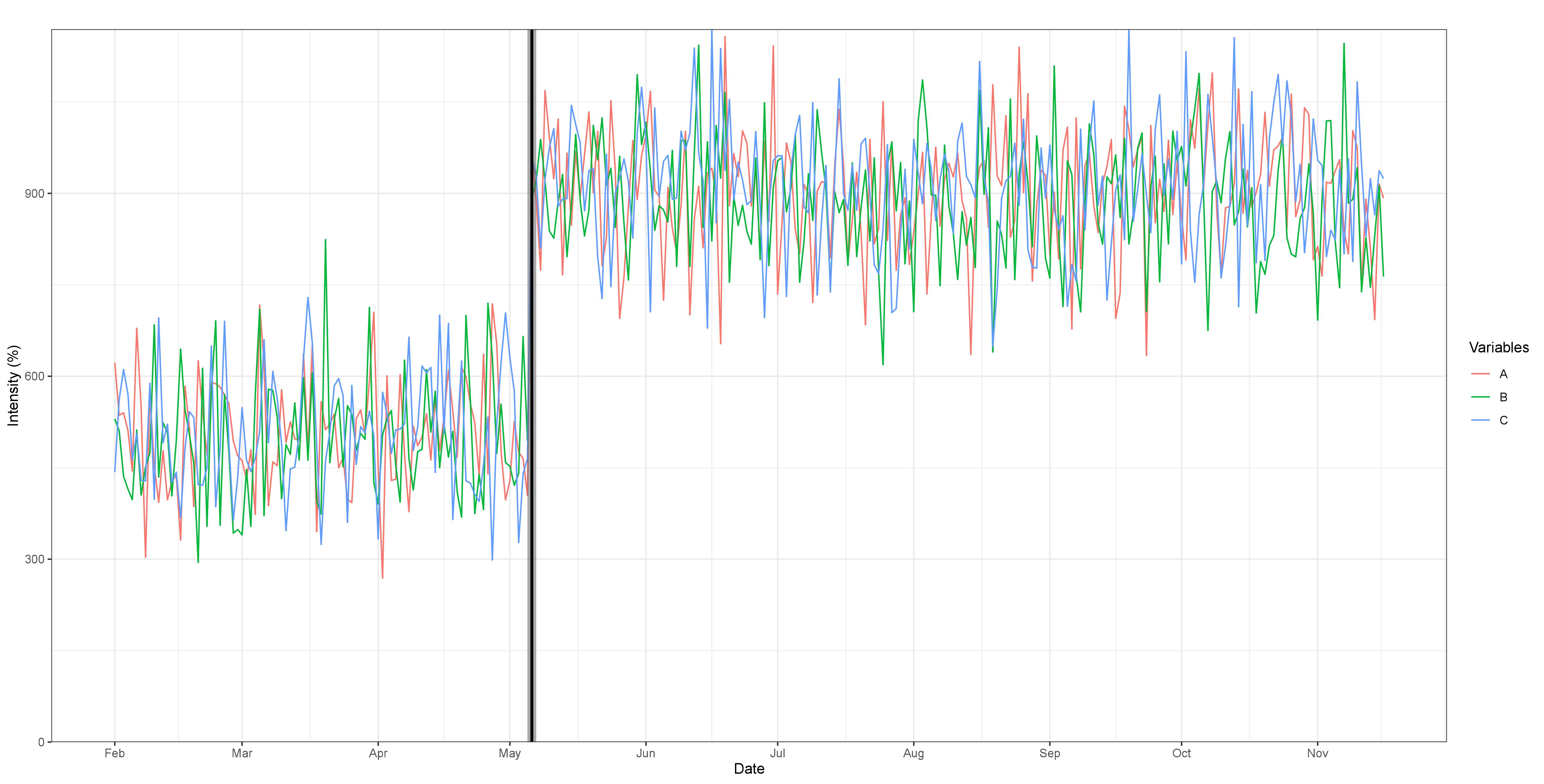
Fig 1. Break detection for three simulated variables experiencing a common break at 35% of the sample, with an intensity parameter of four. The order of the VAR(q) is 1, after selection by the BIC, with no trend or additional covariates added. The break is easy to identify visually and is well captured by the algorithm. Max F-statistic: 159.34, and the confidence intervals for 90%, 95% and 99%, represented by the shaded areas are very concentrated around the break.
Result with five simulated variables
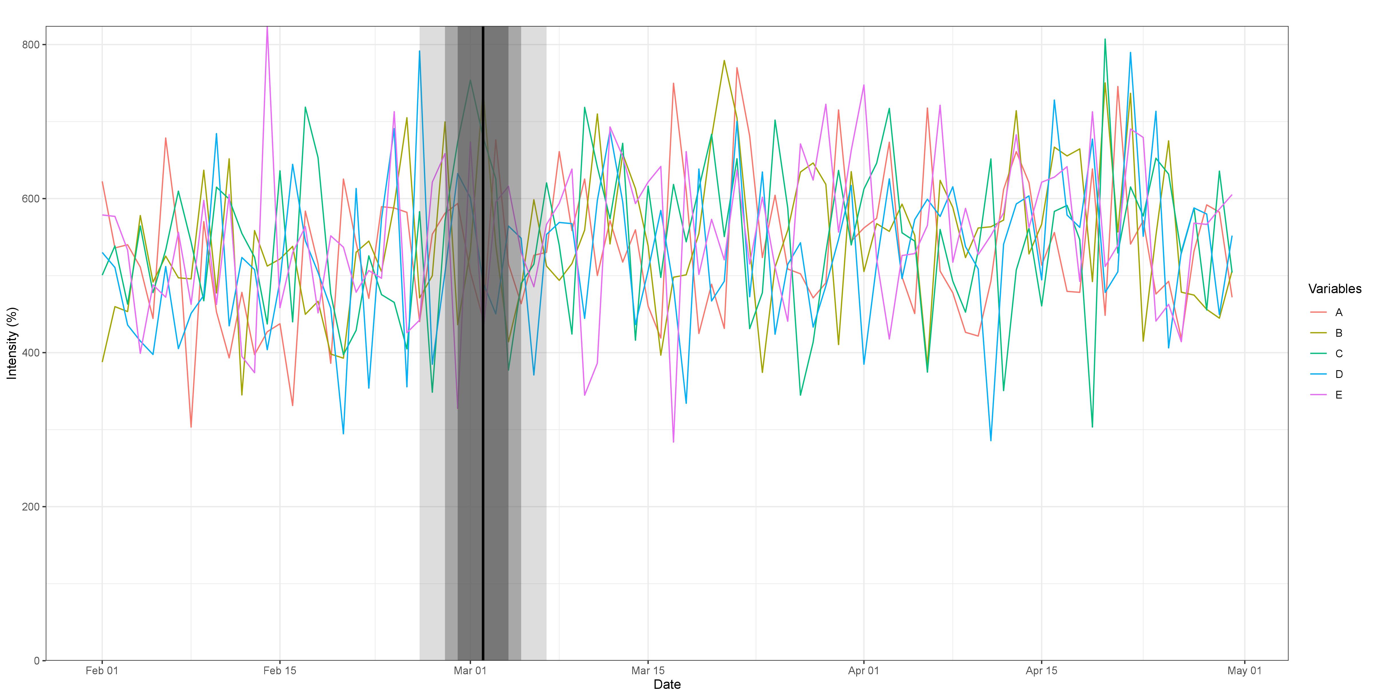
Fig 2. Break detection for five simulated variables experiencing a common break at 35% of the sample, with an intensity parameter of 0.5. The order of the VAR(q) is 1, after selection by the BIC, with no trend or additional covariates added. The break is impossible to detect visually. However, the algorithm accurately captures it. Max F-statistic: 22.72 and the confidence intervals for 90%, 95% and 99%, represented by the shaded areas are much wider.
To get the full working package, including data, you can clone or import the project from my github repository